Reference · 26 entries
Python, plotting and pandas
The pieces of Python the notes’ code uses that go beyond the basics, plus the few plotting and table functions that appear. Click any of them inside a code block to land here.
import … as … · f-string formats: {x:.2f}, {x:>6}, {x:.0%} · Slices: a[:5], a[-1], a[::2], a[::-1] · zip and enumerate · sorted(…, key=lambda …), min and max with key · Comprehensions: [f(x) for x in xs] · Unpacking: a, b = … · assert · try / except · collections.Counter · time.perf_counter · Number spellings: 1e-12, 20_000 · Chained comparisons and in · Sets: set(a) & set(b) · Strings: .split() and .count() · dict.get(key, default) · .copy() · class, self and methods · Functions as values
plt.plot, labels, legend, plt.show · plt.scatter · plt.axhline and plt.axvline · plt.subplots
pd.DataFrame and df["column"] · pd.Series · .loc[rows, columns]
Python beyond the basics
The notes assume plain Python: variables, if, for, functions, lists and dictionaries, and simple f-strings like f"{x}". These are the slightly less common pieces that appear in the code, each in a few lines.
§ import … as …
Imports a library or a function under a shorter name. The short names np (NumPy), pd (pandas) and plt (matplotlib's plotting part) are universal conventions.
Call it as import numpy as np
from module import long_name as short
import numpy as np
import matplotlib.pyplot as plt
from statistics import mean as average
print(np.__name__, plt.__name__)
print(average([1, 2, 3]))outputnumpy matplotlib.pyplot
2
- The notes avoid renaming functions (as mse and so on) in new code, because it makes the code harder to search; you will still see it in other people's code.
§ f-string formats: {x:.2f}, {x:>6}, {x:.0%}
Inside an f-string, a colon after the value says how to print it. .2f means 2 decimal places. A number before it is the total width, so 8.2f pads to 8 characters, which lines up columns. > aligns right, < left. % multiplies by 100 and adds a percent sign. , adds thousands separators.
Call it as f"{value:width.decimalsf}" f"{text:>width}" f"{fraction:.0%}"
x = 3.14159
print(f"{x:.2f}")         # 2 decimals
print(f"[{x:8.2f}]")      # width 8, 2 decimals (padded on the left)
print(f"[{'mean':>6}]")   # text, right-aligned in 6
print(f"{0.3331:.0%}")    # as a percentage
print(f"{1234567:,}")     # thousands separators
print(f"{x = :.3f}") # name and value togetheroutput3.14
[ 3.14]
[ mean]
33%
1,234,567
x = 3.142
- The format goes after a colon inside the braces, not outside: f"{x:.2f}", not f"{x}:.2f".
§ Slices: a[:5], a[-1], a[::2], a[::-1]
a[start:stop] takes elements from start up to but not including stop; leaving one out means 'from the beginning' or 'to the end'. Negative numbers count from the end, so a[-1] is the last element and a[:-1] is everything but the last. A third number is the step: a[::2] takes every second element, a[1::2] every second starting at the second, a[::-1] reverses.
Call it as a[start:stop:step]
a = [0, 10, 20, 30, 40, 50]
print(a[:3])      # first three
print(a[-1])      # last
print(a[:-1])     # all but the last
print(a[::2])     # every second: positions 0, 2, 4
print(a[1::2])    # every second from position 1
print(a[::-1]) # reversedoutput[0, 10, 20]
50
[0, 10, 20, 30, 40]
[0, 20, 40]
[10, 30, 50]
[50, 40, 30, 20, 10, 0]
- The stop position is never included, so a[:3] has three elements.
- The same rules work on NumPy arrays, where a slice is a view: changing it changes the original array.
§ zip and enumerate
zip walks through two (or more) lists side by side, giving one pair at a time. enumerate walks through one list and gives each item together with its position, starting at 0.
Call it as for a, b in zip(list_a, list_b): ...
for i, item in enumerate(items): ...
sizes = [1.0, 1.5, 2.0]
prices = [200, 300, 380]
for size, price in zip(sizes, prices):
    print(size, price)
for i, price in enumerate(prices):
print(i, price)output1.0 200
1.5 300
2.0 380
0 200
1 300
2 380
- zip stops at the shorter list without any warning; pass strict=True to get an error when lengths differ.
§ sorted(…, key=lambda …), min and max with key
sorted returns a new sorted list. key says what to sort by: a small function applied to each item. lambda x: … writes such a small function in one line without a name. min and max take a key the same way. reverse=True sorts from largest to smallest.
Call it as sorted(items, key=lambda item: what_to_sort_by)
words = ["cat", "elephant", "ox"]
print(sorted(words))                            # alphabetical
print(sorted(words, key=lambda w: len(w)))      # by length
print(max(words, key=len))                      # the longest

scores = {"a": 0.9, "b": 0.2, "c": 0.5}
# the keys, highest score first
print(sorted(scores, key=lambda k: scores[k], reverse=True))output['cat', 'elephant', 'ox']
['ox', 'cat', 'elephant']
elephant
['a', 'c', 'b']
- lambda x: len(x) and plain len do the same job as a key; lambda is needed only when the rule is not already a function.
§ Comprehensions: [f(x) for x in xs]
A one-line way to build a list from another: [x * 2 for x in xs] is a loop that collects x * 2 for every x. An if at the end filters. Curly braces with key: value build a dictionary the same way. Without brackets inside a function call, as in sum(x * x for x in xs), it feeds the values one by one without building a list.
Call it as [expression for item in items if condition]
xs = [1, 2, 3, 4]
print([x * 2 for x in xs])                 # list
print([x for x in xs if x % 2 == 0])       # with a filter
print({x: x * x for x in xs})              # dictionary
print(sum(x * x for x in xs)) # straight into sumoutput[2, 4, 6, 8]
[2, 4]
{1: 1, 2: 4, 3: 9, 4: 16}
30
- If the line gets long or has two for parts, a normal loop is easier to read.
§ Unpacking: a, b = …
When something gives back several values at once, you can name them all in one line. The underscore _ is the conventional name for a value you do not need.
Call it as a, b = pair first, _ = pair
pair = (180, 23.3)
w, b = pair
print(w, b)
name, _ = ("slope", 180)     # keep the first, ignore the second
print(name)
x, y = 1, 2
x, y = y, x                   # swap two values in one line
print(x, y)output180 23.3
slope
2 1
- The number of names must match the number of values exactly, or Python raises a ValueError.
§ assert
assert condition checks that something is true and stops the program with an AssertionError if it is not. The notes use it as a built-in self-check: 'this result must equal that one'.
Call it as assert condition, "message if it fails"
import numpy as np
by_loop = sum(a * b for a, b in zip([1, 2, 3], [4, 5, 6]))
by_numpy = np.dot([1, 2, 3], [4, 5, 6])
assert by_loop == by_numpy, "the two ways should agree"
print("checks passed:", by_loop)outputchecks passed: 32
- Compare floating-point results with np.isclose or np.allclose inside the assert, not ==, because tiny rounding differences make == fail.
§ try / except
Runs some code and, if it raises a particular error, runs a fallback instead of crashing. The notes use it to show that an operation fails, for example inverting a matrix that has no inverse.
Call it as try:
risky()
except SomeError as err:
handle(err)
import numpy as np
try:
    # second row = 2 x first row
    np.linalg.inv(np.array([[1.0, 2.0], [2.0, 4.0]]))
except np.linalg.LinAlgError as err:
print("cannot invert:", err)outputcannot invert: Singular matrix
- Catch the specific error you expect, not every error, or real bugs get hidden.
§ collections.Counter
Counts how many times each item appears. most_common(n) gives the n most frequent items with their counts. The notes use it to take a vote among neighbours.
Call it as Counter(items).most_common(1)
from collections import Counter
votes = ["cat", "dog", "cat", "cat", "dog"]
counts = Counter(votes)
print(counts)
print(counts.most_common(1))          # [(item, count)] for the winner
print(counts.most_common(1)[0][0]) # just the winning itemoutputCounter({'cat': 3, 'dog': 2})
[('cat', 3)]
cat
- most_common returns a list of (item, count) pairs, so the winner itself is [0][0].
§ time.perf_counter
Returns the current time in seconds from a precise clock. Call it before and after some code and subtract to see how long the code took.
Call it as start = time.perf_counter(); ...; seconds = time.perf_counter() - start
import time
start = time.perf_counter()
total = sum(range(1_000_000))
seconds = time.perf_counter() - start
print(total, seconds < 1.0)output499999500000 True
- One measurement is noisy; repeat the work a few times and take the best or the average.
§ Number spellings: 1e-12, 20_000
Python lets you write numbers in handier ways. 1e-12 is scientific notation: 1 times 10 to the power -12, a tiny number often added to avoid dividing by zero. Underscores inside a number are ignored and only make it easier to read: 20_000 is 20000.
Call it as 1e-12 2.5e3 1_000_000
print(1e-12)
print(2.5e3)
print(20_000 + 1)
print(1 / (0.0 + 1e-12)) # no division by zerooutput1e-12
2500.0
20001
1000000000000.0
- 1e3 is a float (1000.0), not an int.
§ Chained comparisons and in
a <= b <= c means a <= b and b <= c, the way you would write it in maths. x in items is True when x is one of the items (in a list, a set, a string or a dictionary's keys).
Call it as low <= x <= high x in items
x = 0.7
print(0 <= x <= 1)            # inside the range
print(-1 <= -2 <= 1)          # outside
print(3 in [1, 2, 3])
print("cat" in "concatenate")
print("b" in {"a": 1, "b": 2}) # checks the keysoutputTrue
False
True
True
True
- in on a list checks every element one by one, which is slow for big lists; on a set or dict it is instant.
§ Sets: set(a) & set(b)
A set holds each value at most once, with no order. set(items) removes duplicates. & gives the values in both sets, | the values in either, - the values in the first but not the second. The notes use & to check that two lists share nothing.
Call it as set(a) & set(b) set(a) | set(b) set(a) - set(b)
a = [1, 2, 2, 3]
b = [3, 4]
print(set(a))            # duplicates gone
print(set(a) & set(b))   # in both
print(set(a) | set(b))   # in either
print(len(set(a) & {9})) # 0: nothing sharedoutput{1, 2, 3}
{3}
{1, 2, 3, 4}
0
- {} is an empty dictionary, not an empty set; write set() for an empty set.
§ Strings: .split() and .count()
text.split() cuts a string into a list of words at the spaces. items.count(x) counts how many times x appears in a list (or a string).
Call it as words = text.split() words.count("cat")
text = "the cat sat on the mat"
words = text.split()
print(words)
print(words.count("the"))
print(len(words))output['the', 'cat', 'sat', 'on', 'the', 'mat']
2
6
- split() with no argument also handles several spaces and line breaks; split(" ") does not.
§ dict.get(key, default)
Looks up a key in a dictionary but, instead of failing when the key is missing, gives back the default you chose. Handy for running totals: totals.get(c, 0.0) + x.
Call it as d.get(key, default)
totals = {}
for city, price in [("A", 100), ("B", 300), ("A", 120)]:
    totals[city] = totals.get(city, 0) + price
print(totals)
print(totals.get("Z", 0)) # missing key: the defaultoutput{'A': 220, 'B': 300}
0
- d[key] raises KeyError for a missing key; d.get(key) returns None.
§ .copy()
Makes an independent copy of a list or array. Without it, b = a gives a second name for the same object, so changing b also changes a. NumPy slices are also shared views of the original, so copy before changing them if the original must stay as it was.
Call it as b = a.copy()
import numpy as np
a = np.array([1, 2, 3])
same = a           # another name for the same array
fresh = a.copy()   # a separate array
same[0] = 100
print(a)           # changed through 'same'
fresh[1] = 200
print(a) # unchanged by 'fresh'output[100 2 3]
[100 2 3]
- This is the source of many silent bugs when scaling a column 'in a copy' that was not one.
§ class, self and methods
A class bundles data with the functions that use it. def inside a class defines a method; its first parameter, self, is the object itself, so self.mean = … stores a number on the object and later methods can read it back. This is exactly how scikit-learn's scalers work: fit stores numbers on self, transform reads them.
Call it as class Name:
def method(self, x): ...
import numpy as np

class MeanCentre:
    def fit(self, x):
        self.mean = x.mean()      # remember a number on the object
        return self
    def transform(self, x):
        return x - self.mean      # use the remembered number

step = MeanCentre().fit(np.array([1.0, 2.0, 3.0]))
print(step.mean)
print(step.transform(np.array([10.0])))output2.0
[8.]
- Forgetting self as the first parameter gives 'takes 1 positional argument but 2 were given'.
- return self at the end of fit is what lets you write MeanCentre().fit(x) in one line, as scikit-learn does.
§ Functions as values
In Python a function is a value like any other: you can put it in a list or pass it to another function, then call it later with (). The notes use this to run several fitting methods in one loop.
Call it as for name, fn in [("a", f), ("b", g)]: fn(x)
def double(x):
    return 2 * x

def square(x):
    return x * x

for name, fn in [("double", double), ("square", square)]:
print(name, fn(5))outputdouble 10
square 25
- Write the name without () to pass the function; with () you pass its result instead.
Plotting with matplotlib
matplotlib draws charts. The notes use only a handful of its functions, always through the conventional short name plt. Each example below shows the picture it makes.
§ plt.plot, labels, legend, plt.show
plt.plot(xs, ys) draws a line through the points (xs[0], ys[0]), (xs[1], ys[1]), and so on. Pass label=… and call plt.legend() to name each line. plt.xlabel, plt.ylabel and plt.title write the axis names and the title. plt.show() opens the window (in a notebook the chart appears anyway).
Call it as plt.plot(xs, ys, label="name")
plt.xlabel("x"); plt.ylabel("y"); plt.legend(); plt.show()
import numpy as np
import matplotlib.pyplot as plt

x = np.linspace(0, 3, 50)
plt.plot(x, np.exp(x), label="exp(x)")
plt.plot(x, x ** 2, label="x squared")
plt.xlabel("x")
plt.ylabel("value")
plt.title("Two curves")
plt.legend()
plt.show()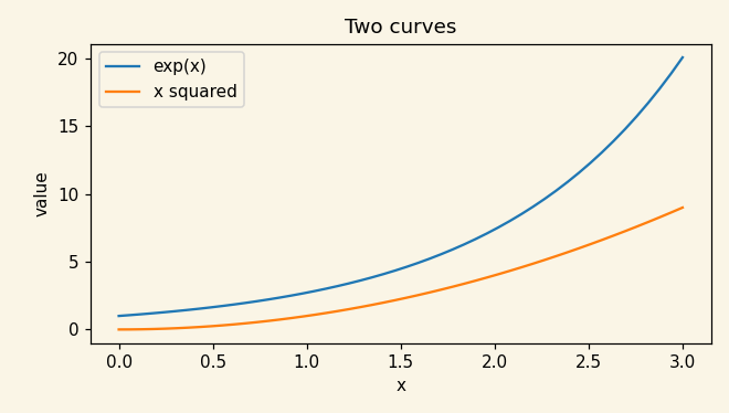
- A smooth curve needs many x values; np.linspace(0, 3, 50) gives 50 of them.
§ plt.scatter
Draws one dot per point, without joining them. Used for data, where joining the dots would suggest an order that is not there.
Call it as plt.scatter(xs, ys)
import matplotlib.pyplot as plt

sizes = [1.0, 1.5, 2.0]
prices = [200, 300, 380]
plt.scatter(sizes, prices)
plt.plot([1.0, 2.0], [203.3, 383.3], label="best line")
plt.xlabel("size (thousand sq ft)")
plt.ylabel("price")
plt.legend()
plt.show()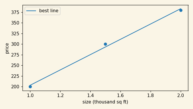
§ plt.axhline and plt.axvline
Draw a straight horizontal line across the whole chart at a given y (axhline), or a vertical one at a given x (axvline). Handy for marking zero, a threshold or a chosen value.
Call it as plt.axhline(y) plt.axvline(x)
import numpy as np
import matplotlib.pyplot as plt

x = np.linspace(-2, 2, 50)
plt.plot(x, x ** 2 - 1)
plt.axhline(0, color="gray")                    # the x-axis
plt.axvline(1, linestyle="--", color="red")     # mark x = 1
plt.show()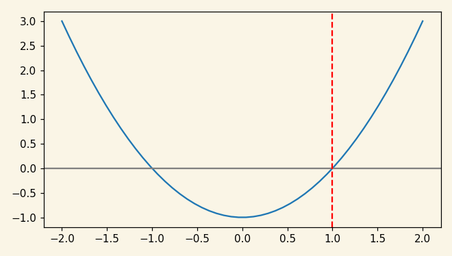
§ plt.subplots
Makes a figure with a grid of separate charts. fig, axes = plt.subplots(1, 2) gives one row of two charts; you then draw on each one through axes[0] and axes[1], whose methods have the same names as plt's (plot, scatter) except that labels use set_xlabel and set_title.
Call it as fig, axes = plt.subplots(rows, cols, figsize=(width, height))
import numpy as np
import matplotlib.pyplot as plt

x = np.linspace(0.1, 5, 50)
fig, axes = plt.subplots(1, 2, figsize=(8, 3))
axes[0].plot(x, np.exp(x))
axes[0].set_title("exp")
axes[1].plot(x, np.log(x))
axes[1].set_title("log")
plt.show()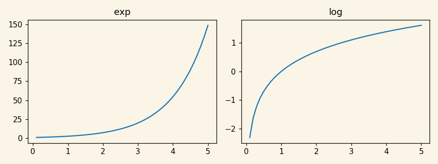
- On an axes object it is set_xlabel and set_title, not xlabel and title.
Tables with pandas
pandas holds a table with named columns, like a spreadsheet in code. The notes use it only where columns have names or mixed types (numbers and categories side by side).
§ pd.DataFrame and df["column"]
A DataFrame is a table: named columns, one row per example, and each column can have its own type (numbers in one, words in another). Build one from a dictionary of column name to values. df["name"] gives one column; df[["a", "b"]] gives a smaller table.
Call it as df = pd.DataFrame({"col": values, ...})
import pandas as pd

df = pd.DataFrame({
    "size": [1.0, 1.5, 2.0],
    "city": ["A", "B", "A"],
    "price": [200, 300, 380],
})
print(df)
print(df["price"].mean())
print(df.shape)
output size city price
0 1.0 A 200
1 1.5 B 300
2 2.0 A 380
293.3333333333333
(3, 3)
- Most scikit-learn steps accept a DataFrame and use its column names; NumPy arrays have no names, only positions.
§ pd.Series
One column on its own: a list of values with a name and an index (the row labels). Taking one column out of a DataFrame gives a Series.
Call it as pd.Series(values, name="col")
import pandas as pd

city = pd.Series(["A", "B", "A", "C"], name="city")
print(city.value_counts())
print(city.nunique())outputcity
A 2
B 1
C 1
Name: count, dtype: int64
3
§ .loc[rows, columns]
Picks rows and columns by their labels. df.loc[0, "price"] is one cell; df.loc[df["city"] == "A", "price"] is the prices of the rows whose city is A.
Call it as df.loc[row_selection, column_selection]
import pandas as pd

df = pd.DataFrame({"city": ["A", "B", "A"], "price": [200, 300, 380]})
print(df.loc[0, "price"])
print(df.loc[df["city"] == "A", "price"].tolist())output200
[200, 380]
- loc uses labels and includes the end of a slice; iloc uses positions and excludes it, like Python.